This is the first part of a two-part examination of what “rural” really means in Oregon and how statistically insignificant (and in all likelihood to become more so) the rural population is today. In Part 1 we examine how much of Oregon is truly rural. In Part 2 we examine the current and future power dynamic between rural and urban Oregon.
There is a dominant narrative of the rural-urban divide in Oregon that often frames our politics, including that of public land management. Like most things in life, it’s not that simple. Superficial news and political analysis tends to be binary: black or white rather than shades of gray. While such shading can provide for more nuance that better informs debate, the world is actually in full color.
A Few Interesting Takeaways
The following are distilled from the analysis that follows:
• The ten true rural counties in Oregon contain just 2.5 percent of the state’s population; 12 counties are metropolitan with 83.5% of the state’s population; and the remaining 13 counties are micropolitan with 14% of the state’s population.
• 18.7 percent of Oregonians live in “rural” settings.
• Four counties are “completely rural,” while 27 counties are “mostly urban.”
• Three Oregon counties are >25% dependent upon farming while eight are similarly dependent upon recreation.
Oregon’s Center of Population Over the Decades
The US Census Bureau uses the concept of the center of population to identify that point in each state where an imaginary, weightless, rigid, and flat (no elevation effects) surface representation would balance if weights of identical size were placed on it so that each weight represented the location of one person. Over the decades, the center of Oregon’s population has hovered mostly in eastern Marion and Linn Counties (Map 1). One might think it would march steadily toward greater Portland, but remember the teeter-totter effect. In this thought exercise, a person in McDermitt on the Nevada-Oregon border and not that far from Idaho will out-balance a very large number of Portlanders.

Map 1. Oregon’s centers of population, 1880–2010. Due to the teeter-totter effect, the movement of that center mostly eastward that peaked in 1900 resulted from the populations in farming counties in north-central and northeastern Oregon being larger relative to the state’s population at the time and larger than their populations today. Source: US Census Bureau
For comparison, the US center of population from 1790 to 2010 is shown in Map 2.

Map 2. US centers of population, 1790–2010, continually on the march toward the Sunbelt (and especially California). Source: US Census Bureau
It will be interesting to see where the US Census Bureau locates Oregon’s center of population after the 2020 census. While the center of population concept is amusing, a more informative determination would be the median balance point where there are an equal number of identically sized people in all directions.
Classifications of Counties
In 2015, the Oregon Office of Economic Analysis issued a report entitled “Rural Oregon: Analyzing Demographic and Economic Trends Across Rural Oregon and a Look Ahead.” To that agency in this report, “rural” means not the western interior counties from Portland to Ashland, or greater Bend (a.k.a. LaBendmondville) (Map 3). But it’s actually a lot more nuanced than that, and bifurcating counties as either urban or rural is hardly illuminating.
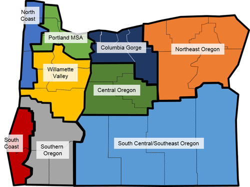
Map 3. So-called "economic regions" identified by the Oregon Office of Economic Analysis, which are more accurately "geographic regions." If you take a closer look, you’ll see that not all the counties in “rural” Oregon are actually rural. Source: Oregon Office of Economic Analysis
Different federal agencies—including the US Census Bureau, the National Center for Health Statistics (NCHS) of the Centers for Disease Control, and the US Department of Agriculture—have more nuanced classification schemes for counties. Table 1 shows how those agencies classify Oregon’s counties.

Table 1. Various Federal County Classification Schemes and the Numbers for Oregon Counties. Sources: US Department of Agriculture, US Census Bureau, National Center for Health Statistics, and Wikipedia
National Center for Health Statistics
The National Center for Health Statistics of the Centers for Disease Control calls true rural counties “noncore” but has the most gradations of non-rural counties, which is important when considering health care delivery and policy (Map 4).
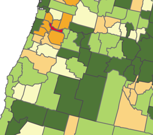
Map 4. NCHS county classifications: red = Large Central Metro, orange = Large Fringe Metro, peach = Medium Metro, cornsilk = Small Metro, light green = Micropolitan, and dark green = Noncore. Source: National Center for Health Statistics
Totaling up the population of Oregon’s counties in each of the six NCHS classifications, we find that the ten Oregon counties (out of thirty-six) that are “noncore” encompass just 2.5 percent of the state’s population (Table 2).
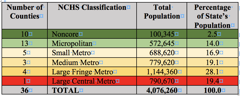
Table 2. Oregon Counties by NCHS Classifications.
The US Census Bureau defines “rural” as what’s left over after defining individual urban areas. It first classifies a variety of kinds of urban areas, including both metropolitan and micropolitan counties. What’s left over doesn’t even get a name or a color (Map 5).

Map 5. US Census Bureau Statistical Areas: dark green = a Metropolitan Statistical Area (MeSA) inside a Combined Statistical Area (CSA); dark brown = a MeSA outside a CSA; light green = a Micropolitan Statistical Area (MiSA) inside a CSA; light brown = a MiSA outside a CSA. The blank spaces on the map are “not urban”—that is, rural. Source: Wikipedia
US Department of Agriculture
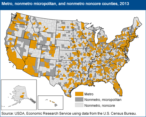
The US Department of Agriculture generally follows the Census Bureau county classifications but coldly calls true rural counties “nonmetro, noncore” (Map 6).

Map 6. USDA county classifications: red = Metro, white = Nonmetro. Source: US Department of Agriculture
The USDA defines “nonmetro” as
- open countryside,
- rural towns (places with fewer than 2,500 people), and
- urban areas with populations ranging from 2,500 to 49,999 that are not part of larger labor market areas (metropolitan areas).
As it prides itself on being in charge of the nation’s rural development, the USDA further parses metro and nonmetro counties into nine different kinds, resulting in the most statistical nuance (Table 3). Depending upon the subsidy program in the farm bill, USDA’s grants can go to “rural” counties with populations up to 50,000, clearly micropolitan and not nonmetro noncore.

Table 3. USDA Rural/Urban Classification Codes for Oregon Counties. Source: USDA
The USDA also assesses the economic dependency of every US county. It has six mutually exclusive categories for any county with a greater than 25 percent economic dependence on that category (Table 4): farming (three Oregon counties), recreation (eight), federal/state government (seven), manufacturing (two), and non-specialized (sixteen). Fortunately, there are no Oregon counties addicted to mining.

Table 4. USDA Economic Dependency Classification of Oregon Counties. Source: USDA
The USDA also ranks the “rurality” of counties (Table 5). Some nonmetro noncore counties are mostly non-rural.

Table 5. USDA Rurality Ratings for Oregon Counties. Source: USDA
The Three Wests
What’s 50 percent better than bifurcation is trifurcation. Headwaters Economics tends to analyze the economics of the American West through an environmental lens parsed by counties (generally very good stuff). One way it parses the West is based on transportation access—especially, but not exclusively, commercial air service (Map 7). Counties either have it, are next to it, or are not close.

_of_the_United_States_and_Puerto_Rico,_Feb_2013.gif)
Map 7. The “Three Wests” based on transportation access. Headwaters Economics trifurcated western counties based on ease of access to transportation. Much of “rural” Oregon actually consists of “connected counties.” (I would make Douglas County yellow, as it is bisected by Interstate 5 and for most is an hour’s drive to the Eugene airport.) Source: Headwaters Economics
This post continues with Part 2 next week.